Exploring the Power of AutoEncoders in Deep Hyperspectral Image Analysis

The AutoEncoders are a classic example of an unsupervised learning technique that utilizes artificial neural networks in representation learning. They are among the earliest deep learning methods considered as the building blocks in deep hyperspectral image analysis.

The Mechanics of Training AutoEncoders

A simple autoencoder is a feed-forward, non-recurrent neural network with three layers, i.e., the input, the hidden, and the output layers, as shown in Figure below.

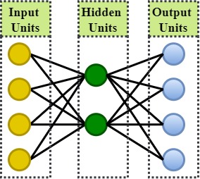
Training an AutoEncoder: The Encoding and Decoding

Like any other feed-forward neural network, the autoencoders train through backpropagation of the error function. The training process in the autoencoder is divided into the encoding and decoding sub-processes.

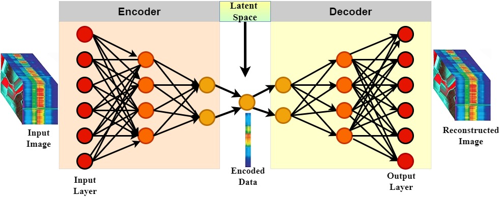
During the encoding process, the autoencoder is explicitly forced to map input image p with n units to the hidden units m. Each input is connected to all hidden neurons. The resultant image h∈R^m at the hidden layer, preservers later preserve only the most relevant aspects of the input data in the data code and are usually referred to as the code, a latent representation, or latent variables. Depending on the structure of the hidden layer, autoencoders can be classified as overcomplete, sparse, denoising, or incomplete. Each type serves a unique purpose:

Overcomplete Autoencoder

If the dimension of the hidden image h∈R^m is larger than or the same as that of the input image p∈R^m, such that m ≥ n, then there is no constraint on the hidden layer as the autoencoder will provide a one-to-one mapping to perfectly mirror the input signals at the output. In this case, the autoencoder learns nothing, thus rendering it useless hence referred to as an overcomplete autoencoder. The following two approaches were developed to solve the identical mapping challenge:

• Adding a normalization term to the reconstruction error to produce a sparse representation with a certain degree of noise immunity and a near zero network parameters resulting in the development of a sparse autoencoder.
• Adding noise to the input data and train the network to remove it, resulting in a robust representation of the original input resulting in the development of a denoising autoencoder. During encoding, the denoising autoencoder adds some noise p_noise to the input p, and during decoding, the noise p_noise that was added during encoding is removed, hence producing a powerful hidden representation of the input p.

Incomplete autoencoder

If the dimensionality of the hidden layer h∈R^m is lower than that of the input layer p∈Rⁿ, such that m < n results in the development of an incomplete autoencoder. At this point, the autoencoder acts as a dimensionality reduction technique. The autoencoders are typically forced to reconstruct their inputs from image h by mapping h∈ R^m to p∈Rⁿ during the decoding process to produce the output image q which in most cases is not a perfect mirror of the input image p due to the reconstruction error. To minimize the reconstruction error/loss (‖p-q‖²), incomplete autoencoders are trained to apply various approaches.

Autoencoders can be used for dimensionality reduction by encoding input data into a compressed representation, which captures the most important features, and then reconstructing the original data from this reduced form.

The Rise of The Stacked Autoencoders (SAEs) in Deep Hyperspectral Image Classification

When autoencoders were first used in hyperspectral image feature learning, they only extracted spectral features and were unable to capture spatial features. However, the true magic happens when they are stacked to form the stacked autoencoders (SAEs) as shown in Figure below.

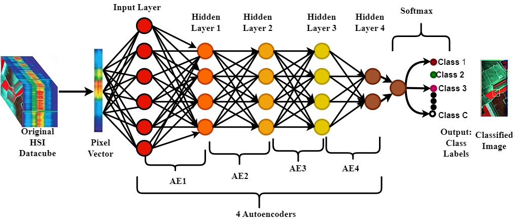
The stacked autoencoders (SAEs) consist of an input layer, several hidden layers, and an output layer to learn more discriminative features as shown above. To perform classification, the final hidden layer is typically linked to a softmax layer, which produces the probability distribution for each potential class. By stacking multiple autoencoders, each layer builds upon the previous one, such that, the output of one autoencoder layer becomes the input of the next auto-encoder layer which enhances the network’s ability to learn more intricate and discriminative features. Since fully connected networks like the stacked autoencoders SAE (and its variants) only accept vectorized input data, it extracted spectral-spatial features from the HSI datacube by flattening the neighboring spatial pixels into a 1-D input and stacking it with the original spectral vector.

Innovative Techniques and Applications

Researchers have continuously pushed the boundaries of what autoencoders can achieve. For instance, Sun et al. (2017) proposed a network that integrates spectral and spatial data, significantly boosting classification performance. They introduced innovative training strategies and pooling methods that allow the network to better handle confusing samples and improve overall accuracy. Another notable advancement comes from Pan et al. (2019), who developed a two-stream network. One stream focuses on spectral information, while the other captures spatial features. By fusing these streams and utilizing SVM classification, they achieved remarkable results in predicting class labels.

Conclusion

Autoencoders are a powerful tool in the deep learning arsenal, particularly for tasks requiring complex data interpretation like hyperspectral image analysis. By continuously refining these networks and exploring new techniques, researchers unlock even greater potential, paving the way for more accurate and efficient data analysis.

Further Reading

Chen, Y., Jiang, H., Li, C., Jia, X., & Ghamisi, P. (2016). Deep Feature Extraction and Classification of Hyperspectral Images Based on Convolutional Neural Networks. IEEE Transactions on Geoscience and Remote Sensing, 54(10), 6232–6251. https://doi.org/10.1109/TGRS.2016.2584107

Haron Tinega, Chen, E. and Divinah Nyasaka (2023). Improving Feature Learning in Remote Sensing Images Using an Integrated Deep Multi-Scale 3D/2D Convolutional Network. Remote Sensing, 15(13), pp.3270–3270. doi:https://doi.org/10.3390/rs15133270.

Haron Tinega, Chen, E., Ma, L., Divinah Nyasaka and Mariita, R.M. (2022). HybridGBN-SR: A Deep 3D/2D Genome Graph-Based Network for Hyperspectral Image Classification. Remote Sensing, 14(6), pp.1332–1332. doi:https://doi.org/10.3390/rs14061332.

Haron Tinega, Chen, E., Ma, L., Mariita, R.M. and Divinah Nyasaka (2021). Hyperspectral Image Classification Using Deep Genome Graph-Based Approach. Sensors, 21(19), pp.6467–6467. doi:https://doi.org/10.3390/s21196467.

Li, S., Song, W., Member, S., Fang, L., & Member, S. (2019). Deep Learning for Hyperspectral Image Classification : An Overview. IEEE TRANSACTIONS ON GEOSCIENCE AND REMOTE SENSING, 57(9), 6690–6709. https://doi.org/10.1109/TGRS.2019.2907932

Sun, X., Zhou, F., Dong, J., Gao, F., Mu, Q., & Wang, X. (2017). Encoding Spectral and Spatial Context Information for Hyperspectral Image Classification. IEEE Geoscience and Remote Sensing Letters, 14(12), 2250–2254.

Tao, C., Pan, H., Li, Y., & Zou, Z. (2015). Unsupervised Spectral-Spatial Feature Learning With Stacked Sparse Autoencoder for Hyperspectral Imagery Classification. IEEE Geoscience and Remote Sensing Letters, 12(12), 2438–2442. https://doi.org/10.1109/LGRS.2015.2482520